Code
library(tidyverse)
theme_set(theme_void() + theme(legend.position = 'none'))

# I will go parallel a little later; set up my computer for this
library(future)
library(furrr)A Computational Journey through Parameter Spaces
Abhirup Moitra
February 10, 2024

“The grand aim of all science is to cover the greatest number of empirical facts by logical deduction from the smallest number of hypotheses or axioms.” - Albert Einstein
This research article delves into the fascinating realm of strange attractors, as elucidated in Julien C. Sprott’s seminal work. The availability of Sprott’s book as a free downloadable resource has facilitated widespread exploration of these complex phenomena. Noteworthy features include a profusion of captivating imagery and accompanying source code, rendering the subject accessible to enthusiasts adept in basic programming. A key focus of this research lies in the exploration of strategies to navigate the vast parameter spaces inherent to strange attractors. Drawing insights from the techniques expounded in Sprott’s text, the paper sheds light on methodologies to discern aesthetically pleasing patterns within these intricate systems. Central to our investigation is the implementation of a two-dimensional quadratic map, governed by a set of twelve parameters.
\[ \begin{align*}x_{n+1} &= a_1 + a_2 x_n + a_3 x_n^2 + a_4 x_n y_n + a_5 y_n + a_6 y_n^2 \\y_{n+1} &= a_7 + a_8 x_n + a_9 x_n^2 + a_{10} x_n y_n + a_{11} y_n + a_{12} y_n^2\end{align*} \]
Through judicious selection and manipulation of these parameters, we embark upon a visual journey, culminating in the generation of captivating images. The paper offers insights into the nuances of parameter selection and its profound impact on the resultant visualizations. By leveraging Sprott’s foundational work and building upon it with novel implementations in the R programming language, this paper contributes to the ongoing discourse surrounding strange attractors. It underscores the symbiotic relationship between mathematical theory and computational implementation in unraveling the mysteries of chaotic dynamical systems. In conclusion, this research serves as a testament to the enduring relevance and beauty of strange attractors, offering both theoretical insights and practical methodologies for enthusiasts and researchers alike.
In order to generate an initial illustrative depiction, a deliberate selection of parameter values for the twelve variables was undertaken. The determination of ‘suitable’ values, a concept meriting further elucidation, was pivotal in this process. Subsequently, a series of computational steps were executed, culminating in the generation of visual representations elucidating the emergent patterns. These results were then meticulously plotted for comprehensive analysis and interpretation.
1.1 Code
This code segment is written in R and serves to set up the environment for subsequent data visualization and parallel processing tasks.
library(tidyverse): This line loads the tidyverse package, which is a collection of R packages designed for data manipulation and visualization. It includes popular packages such as ggplot2, dplyr, and tidyr.
theme_set(theme_void() + theme(legend.position = 'none')): This line sets the default theme for plots using ggplot2 to a blank theme (theme_void()) with no axes or background, and also removes the legend from plots. This ensures that plots generated later will have a clean appearance without unnecessary clutter.
library(future): This line loads the future package, which provides tools for parallel computing in R.
library(furrr): This line loads the furrr package, which builds on top of future and provides a user-friendly interface for parallel programming in R.
The primary function, denoted as quadratic_2d(), is designed to accept a vector denoted as ‘a’, encapsulating the twelve parameters pertinent to the two-dimensional quadratic map. Additionally, this function requires an input pair comprising the coordinates along the x and y axes, designated as an \((x,y)\) pair, to compute and generate the subsequent step forward within the dynamical system.
1.2 Code
This code defines a function named quadratic_2d. This function takes three arguments: a, xn, and yn.
a is expected to be a vector containing twelve parameters.
xn represents the current value along the x-axis.
yn represents the current value along the y-axis.
Within the function, two new variables xn1 and yn1 are computed using the supplied parameters a and the current coordinates xn and yn according to the formulas provided. These formulas represent the calculation of the next step forward in a two-dimensional quadratic map. Finally, the function returns a vector containing the newly computed values xn1 and yn1.
We have further implemented a function, termed iterate(), to systematically traverse through iterations within the defined dynamical system. The iterate() function facilitates the accumulation of outcomes, yielding a comprehensive list of points visited throughout the execution of the map over a specified number of iterations. Utilizing a set of parameters, designated as ‘a’, this function orchestrates the generation of what is commonly referred to as the Hénon map, as delineated below.
1.3 Code
iterate <- function(step_fn, a, x0, y0, iterations) {
x <- rep(x0, iterations)
y <- rep(y0, iterations)
for(n in 1:(iterations - 1)) {
xy <- step_fn(a, x[n], y[n])
x[n+1] <- xy[1]
y[n+1] <- xy[2]
}
tibble(x = x, y = y) %>%
mutate(n = row_number())
}
henon_a <- c(1, 0, -1.4, 0, 0.3, 0, 0, 1, 0, 0, 0, 0)
iterate(step_fn = quadratic_2d, a = henon_a,
x0 = 0, y0 = 0, iterations = 5000) %>%
ggplot(aes(x, y)) +
geom_point(size = 0, shape = 20, alpha = 0.2) + # Plot a pixel for each point
coord_equal()
This code defines a function named iterate and subsequently utilizes it to generate and visualize a trajectory within the Hénon map using the specified parameters.
The iterate function takes five arguments: step_fn, a, x0, y0, and iterations.
step_fn represents the function responsible for computing the next step in the iteration process.
a denotes the parameters governing the dynamical system.
x0 and y0 signify the initial coordinates from which the iteration begins.
iterations indicates the total number of iterations to perform.
Within the iterate function, two vectors x and y are initialized with repeated values of x0 and y0, respectively. Subsequently, a loop iterates through each step, invoking the step_fn function to compute the next coordinates based on the parameters a and the current x and y values. These computed coordinates are stored in the x and y vectors for subsequent iterations.
Upon completion of the iteration process, a tibble (data frame) is constructed with columns x and y, representing the trajectory, and an additional column n denoting the iteration number.
The subsequent code snippet utilizes the iterate function to generate a trajectory within the Hénon map, specifically employing the parameters defined in the henon_a vector. The trajectory is initialized from the origin (0, 0) and spans 5000 iterations.
The resulting trajectory is then visualized using ggplot2, with each point represented as a pixel on the plot. The geom_point function is employed to plot the points, while coord_equal() ensures that the aspect ratio of the plot remains consistent. Additionally, the points are rendered with minimal size (size = 0) and transparency (alpha = 0.2), facilitating the visualization of the entire trajectory.
In the context of a 2D quadratic map, it is imperative to acknowledge the intricate nature of parameter selection, wherein a staggering twelve parameters necessitate discerning choices. However, not all parameter configurations yield meaningful or visually captivating outcomes.
Distinct categories of plots emerge contingent upon the specific parameter combinations:
Converging: These plots depict trajectories culminating in fixed points, offering little in terms of visual intrigue or dynamical complexity.
Run-away: Characterized by trajectories spiraling towards infinity, these plots similarly lack substantive interpretive value.
Chaotic: Representing the focal point of interest, chaotic plots exhibit intricate, non-linear behavior, embodying the essence of dynamical complexity.
In pursuit of chaotic behavior, parameter values within a bounded range typically exhibit the greatest propensity for generating visually compelling results. Empirical observations suggest that parameter values ranging between -1.5 and 1.5, incremented by steps of 0.01, offer a favorable likelihood of inducing chaotic behavior. Nonetheless, even within this bounded domain, the sheer combinatorial magnitude remains daunting, with an estimated 10^70 distinct parameter configurations.
To mitigate the arduous task of manually sifting through this vast parameter space, computational techniques can be harnessed. A fundamental understanding of chaotic systems reveals two salient characteristics:
Divergence: Nearby points within the system tend to diverge from each other over successive iterations, precluding convergence towards a fixed point.
Finite Bounds: Despite the tendency to diverge, trajectories within chaotic systems remain bounded, exhibiting periodic oscillations rather than unbounded divergence towards infinity.
Guided by these insights, an algorithmic approach emerges: iteratively track the trajectories of two adjacent points within the parameter space. At each iteration, evaluate the change in distance between these points and ascertain whether it increases or decreases. Subsequently, aggregate these observations over multiple iterations, discerning whether the average ratio of post-iteration to pre-iteration distances exceeds unity, indicative of divergent behavior. This algorithmic framework enables automated identification and characterization of chaotic parameter configurations, alleviating the burden of manual exploration within the parameter space.
In mathematical terms, let us define the parameter \(L\) as follows:
\[ L = \sum_{l} \frac{\log_2 (d_n + 1)}{d_n / N} \]
Here, \(d\) represents the distance between two successive points, and \(N\) denotes the total number of points evaluated. Notably, given the utilization of logarithmic transformations, our criterion for chaotic behavior hinges upon the condition \(L>0\) (owing to the property that \(2^0=1\)).
Subsequently, upon satisfying the condition \(L>0\) and observing that the \(xy-\) coordinates do not exhibit unbounded growth (remaining within a finite range, for instance, within the interval \(±\) one million), we identify a set of parameters exhibiting chaotic behavior. Let’s implement a function to calculate \(L\).
1.4 Code
L <- function(step_fn, a, x0, y0, iterations = 1000) {
# Really, put the point nearby and see what happens
nearby_distance <- 0.000001
xy <- c(x0, y0)
xy_near <- xy + c(nearby_distance, 0)
# Collect the log distance ratios as we iterate
sum_log_distance_ratios <- 0
for (n in 1:iterations) {
xy <- step_fn(a, xy[1], xy[2])
xy_near <- step_fn(a, xy_near[1], xy_near[2])
new_distance = sqrt((xy[1] - xy_near[1])^2 + (xy[2] - xy_near[2])^2)
if (new_distance == 0) {
# The points have converged
return (-Inf)
}
if (abs(new_distance) == Inf) {
# The points have run away
return (Inf)
}
# Move near point after xy
# We put the near point just behind in the direction that they differ
angle = atan2(xy_near[2] - xy[2], xy_near[1] - xy[1])
xy_near <- c(xy[1] + nearby_distance * cos(angle),
xy[2] + nearby_distance * sin(angle))
sum_log_distance_ratios = sum_log_distance_ratios + log2(new_distance / nearby_distance)
}
sum_log_distance_ratios / iterations
}This code defines a function named L that computes the value of the parameter \(L\), as described earlier. The function takes five arguments: step_fn, a, x0, y0, and iterations, with iterations defaulting to \(1000\). Within the function, a nearby distance variable is initialized to a very small value, allowing for the creation of a nearby point during the iteration process.
Subsequently, the function iterates through a loop for the specified number of iterations. At each iteration, it computes the distance between the current point and the nearby point, updates the nearby point using the step_fn function, and calculates the new distance between the updated points. If the distance between the points becomes zero, indicating convergence, the function returns negative infinity. Conversely, if the distance becomes infinite, indicating divergence, the function returns positive infinity.
Finally, the function computes the sum of the logarithmic distance ratios over all iterations and divides it by the total number of iterations to obtain the average value of \(L\), which is then returned. Overall, this function encapsulates the algorithmic approach outlined earlier for assessing chaotic behavior within the dynamical system.
Applying this computational methodology to a selection of parameter sets, we aim to assess the chaotic behavior inherent within the Hénon map, as established in prior literature.
When all parameters are set to zero, the iterative process converges to the fixed point located at the origin, denoted as \((0, 0).\)
With the requisite components integrated into the computational framework, a comprehensive exploration ensues wherein a sizable array of parameter sets is randomly generated. From this pool, only those exhibiting characteristics indicative of chaotic behavior are selectively retained for further analysis.
1.5 Code
This code segment initiates a computational procedure aimed at identifying parameter sets conducive to chaotic behavior within the context of a 2D quadratic map. The set.seed(1) function ensures reproducibility by fixing the random number generator seed.
Subsequently, a tibble named df is generated, containing a sequence of integers labeled as pattern ranging from 1 to 1000. Each integer is associated with a corresponding set of twelve parameters denoted as a, generated using the runif() function to randomly sample values within the interval [-1.5, 1.5], rounded to two decimal places.
The map() function from the purrr package is then employed to apply the quadratic_2d function iteratively to each parameter set a, alongside initial coordinates \((0, 0)\), to compute the value of the parameter \(L\). This results in the creation of a new column L_val within the dataframe df, containing the calculated values of \(L\).
Subsequently, the dataset is filtered to retain only those parameter sets for which the computed \(L\) value exceeds zero, indicative of chaotic behavior.
Finally, the resulting dataframe df is printed to the console, providing a tabular representation of the parameter sets that exhibit chaotic dynamics within the 2D quadratic map.
In this analysis, we identify a subset of 17 candidate parameter sets characterized by an \(L\) value exceeding zero, indicative of potential chaotic behavior within the dynamical system. While it remains plausible that some of these sets may exhibit unbounded divergence with further iterations, our initial screening process effectively reduces the pool of parameter sets necessitating computation and inspection.
To harness the potential of these promising parameter configurations, a subsequent iteration is conducted with an increased number of iterations. Additionally, to facilitate comparative analysis and visualization, the \(xy-\) coordinates are normalized to a range from \(0\) to \(1\), ensuring uniform scaling across all plotted trajectories
1.6 Code
normalize_xy <- function(df) {
range <- with(df, max(max(x) - min(x), max(y) - min(y)))
df %>%
mutate(x = (x - min(x)) / range,
y = (y - min(y)) / range)
}
render_grid <- function(df, iterations) {
df %>%
mutate(xy = map(a, ~ iterate(quadratic_2d, ., 0, 0, iterations))) %>%
# Remove those who have grown very large / might run away
filter(map_lgl(xy, function(d) with(d, all(abs(x) + abs(y) < 1e7)))) %>%
mutate(xy = map(xy, normalize_xy)) %>%
unnest(xy) %>%
ggplot(aes(x, y)) +
geom_point(size = 0, shape = 20, alpha = 0.1) +
coord_equal() +
facet_wrap(~ pattern)
}
df %>%
render_grid(5000)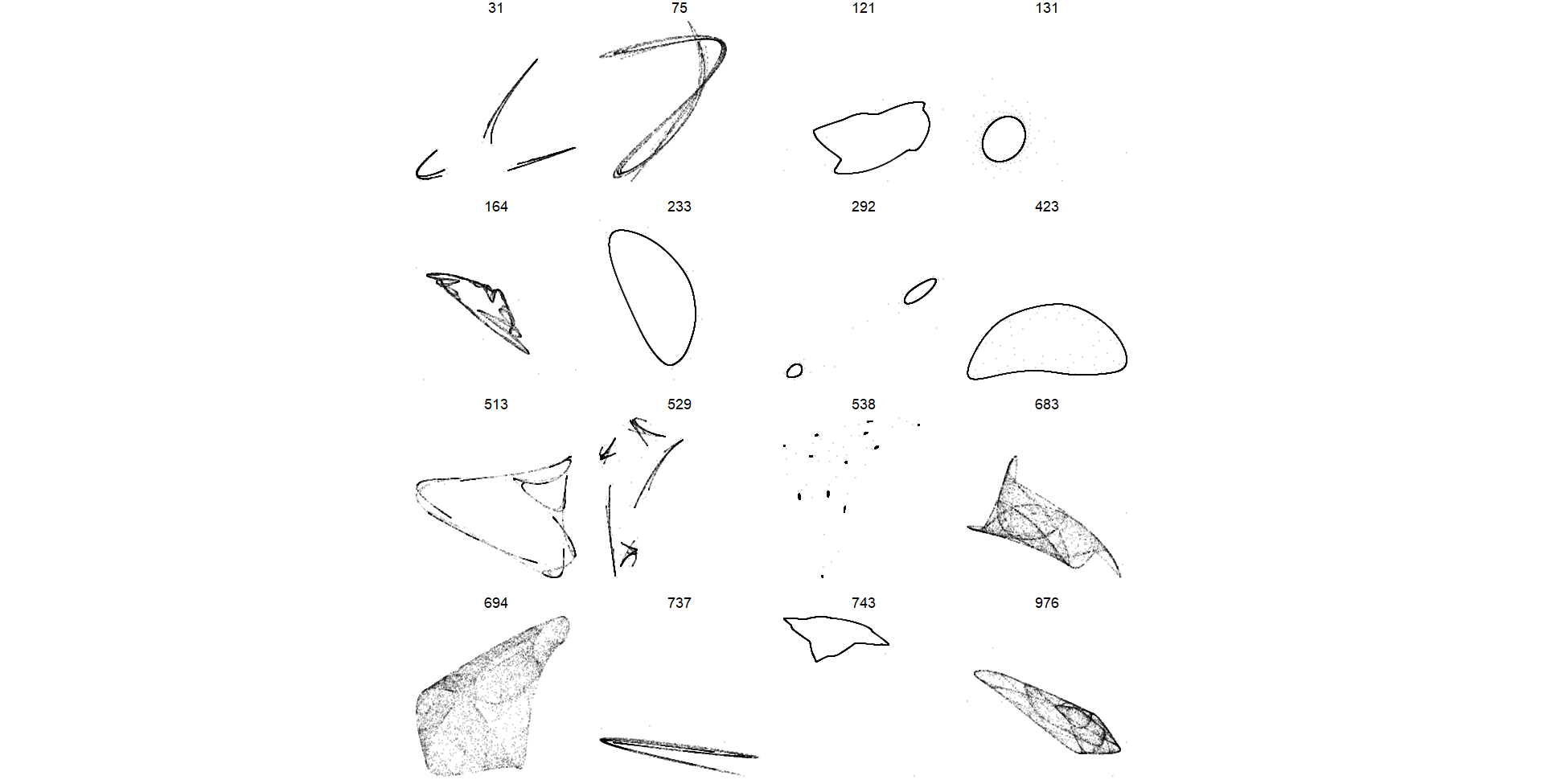
This code performs two main tasks: normalizing \(xy-\) coordinates and rendering a grid of plots representing trajectories of parameter sets in a 2D quadratic map.
normalize_xy function: This function takes a dataframe df containing \(xy-\) coordinates and normalizes these coordinates to a range from 0 to 1. It first calculates the range of values in both \(x\) and \(y\) dimensions. Then, it updates the dataframe by transforming each \(x\) and \(y\) coordinate using the formula \(\frac{x- \text{min}(x)}{\text{range}}\) and \(\frac{y-\text{min(y)}}{\text{range}}\), respectively.
render_grid function: This function renders a grid of plots representing trajectories of parameter sets in a 2D quadratic map. It takes two arguments: df, a dataframe containing parameter sets, and iterations, the number of iterations to compute the trajectories.
It first computes the trajectories for each parameter set using the iterate function.
Next, it filters out trajectories that have grown very large or might run away, ensuring that only stable trajectories are plotted.
Then, it normalizes the \(xy-\) coordinates of each trajectory using the normalize_xy function.
Finally, it creates a grid of plots using ggplot2, with each plot representing the trajectory of a parameter set. The plots are arranged in a grid format, with each row corresponding to a different parameter set (pattern).
The last part of the code applies the render_grid function to the dataframe df with a specified number of iterations (5000), generating and displaying the grid of plots representing the trajectories of parameter sets in the 2D quadratic map.
Despite the presence of some trajectories exhibiting periodic behavior deemed less visually appealing, we proceed to render one trajectory with enhanced quality for thorough analysis:
1.7 Code
Pattern 423: This code filters the dataframe df to retain only the observations corresponding to pattern number 423. It then calls the render_grid function with this filtered subset of data and a specified number of iterations (100,000). The render_grid function generates and renders a plot representing the trajectory of parameter sets associated with pattern 423 in the 2D quadratic map, using a larger number of iterations to capture finer details of the trajectory.
Pattern 683: This code selects a subset of data from the dataframe df where the pattern variable is equal to 683. It then proceeds to render a grid of plots representing trajectories associated with this specific pattern, using a large number of iterations (100,000) to capture intricate details of the trajectory behavior.
Pattern 694: This code filters the dataframe df to extract observations corresponding specifically to pattern number 694. Subsequently, it generates a grid of plots representing trajectories associated with this pattern. The function utilizes a significant number of iterations (100,000) to ensure thorough examination and capture intricate details of the trajectory dynamics.
Pattern 75: This code filters the dataframe df to extract observations corresponding exclusively to pattern number 75. Subsequently, it generates a grid of plots representing trajectories associated with this specific pattern. Utilizing a substantial number of iterations (100,000), the function aims to comprehensively analyze and depict the intricate details of the trajectory dynamics for this particular pattern
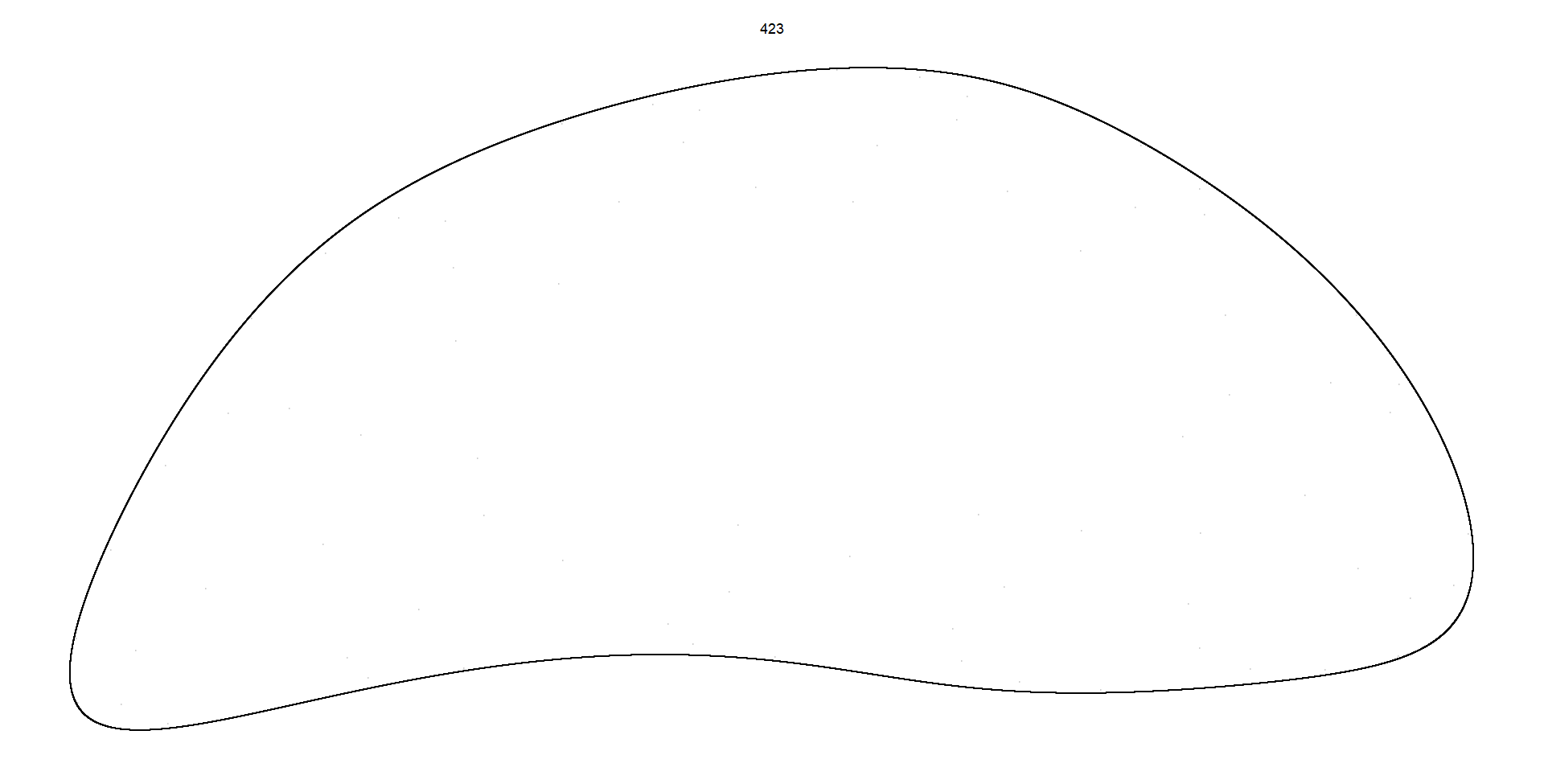
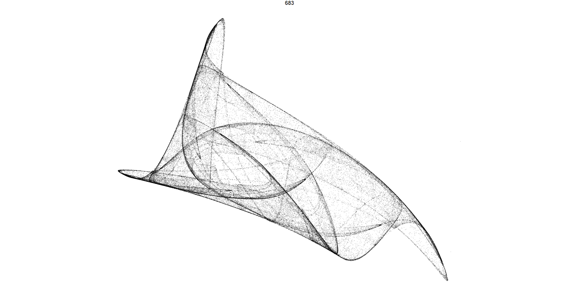
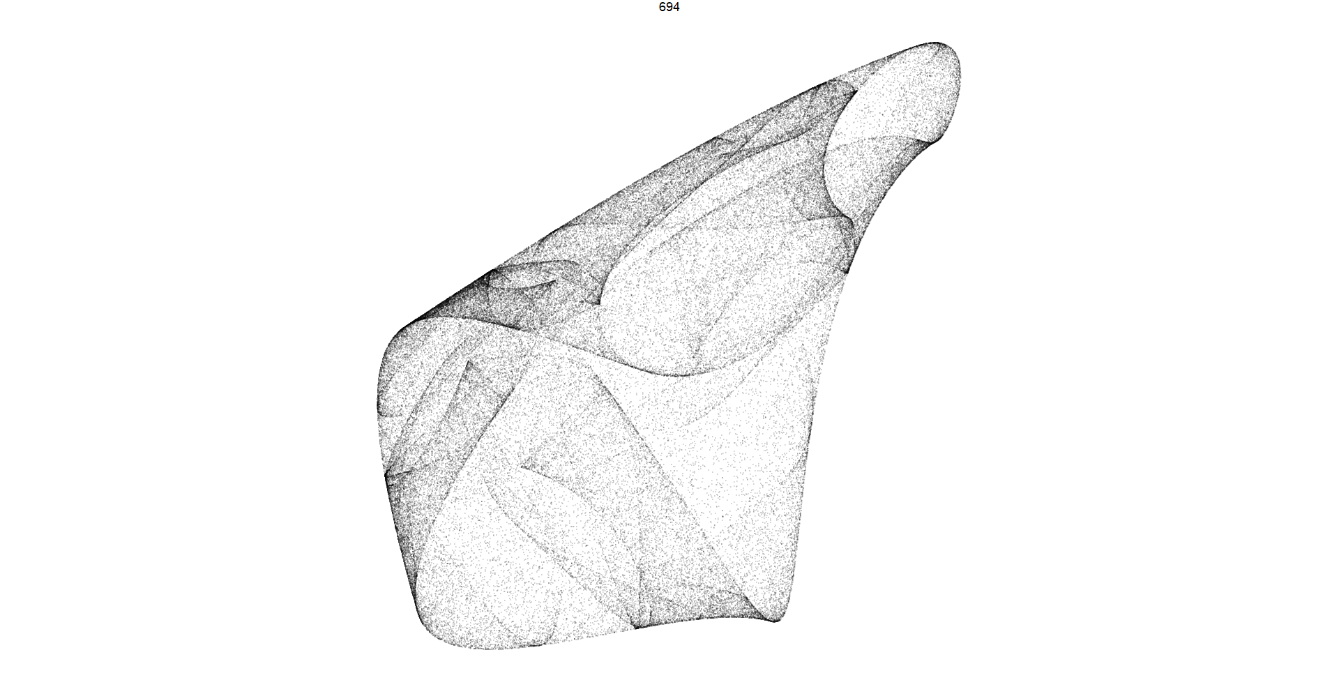
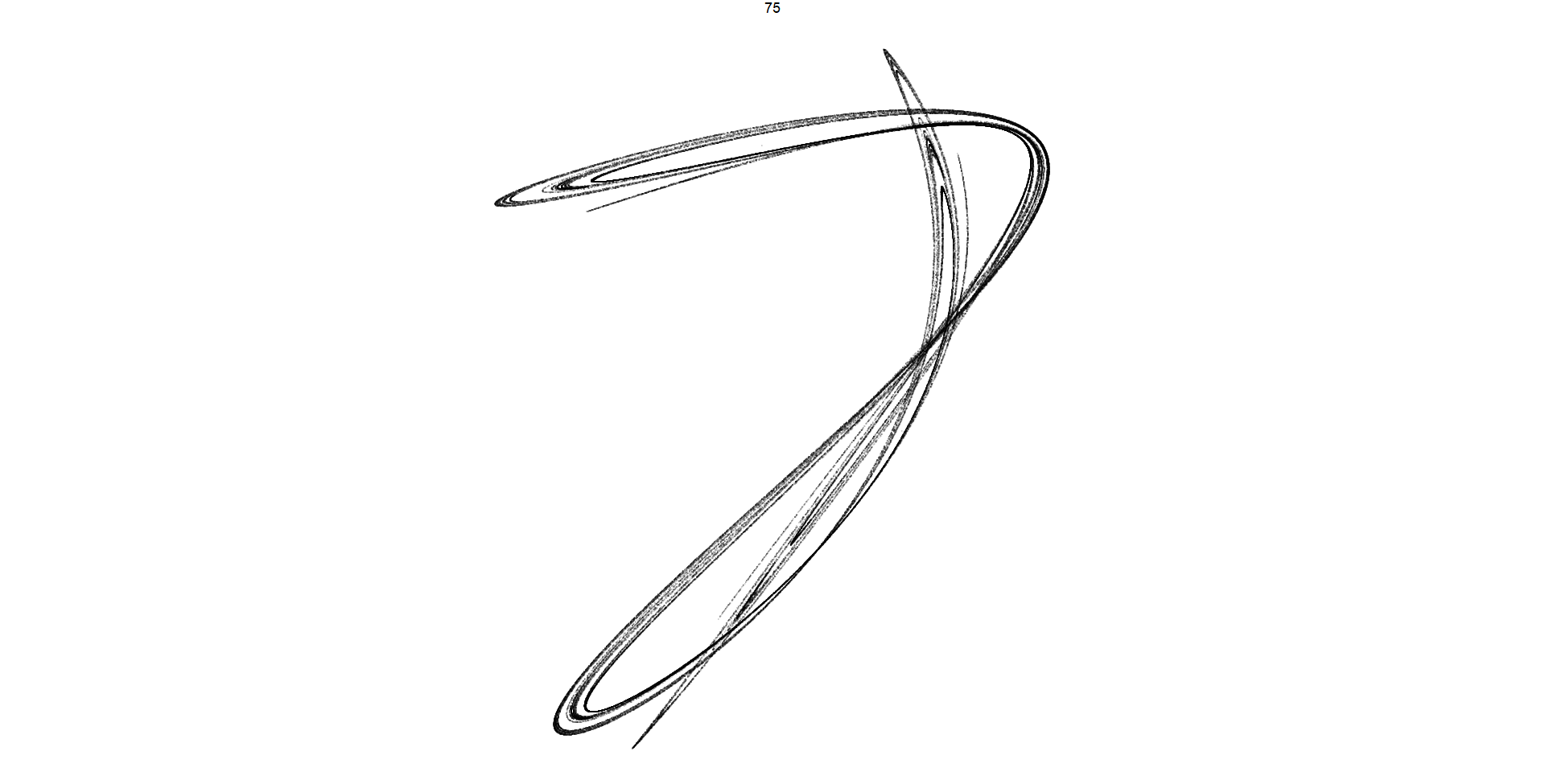
We employ a flexible approach to adjust the rendering of identified patterns, aiming to enhance visualization effectiveness. A notable technique involves aggregating individual points into grid-based ‘bins,’ facilitating efficient visualization by quantifying the density of points within each cell. This method allows us to map the count of points to color and transparency values, offering insights into the spatial distribution of trajectories.
To expedite computational processing, we implement parallelization techniques for data generation. By distributing the iterations evenly across the cores of the CPU, computational workload is efficiently managed. Additionally, we introduce slight variations in starting points for each thread, resulting in parallel execution of iterations across multiple cores. Given the nature of attractors to converge trajectories towards more frequently visited regions regardless of initial starting points, the concurrent execution of multiple paths remains imperceptible.
1.8 Code
render_print_data <- function(a, iterations, gridsize) {
CPU_cores <- parallel::detectCores()
tibble(thread = 1:CPU_cores) %>%
mutate(x0 = runif(length(thread), -0.1, 0.1),
y0 = runif(length(thread), -0.1, 0.1)) %>%
mutate(xy = future_pmap(., function(x0, y0, ...) iterate(quadratic_2d, a, x0, y0, iterations / CPU_cores))) %>%
unnest(xy) %>%
# Normalize
mutate(range = max(max(x) - min(x), max(y) - min(y))) %>%
mutate(x = (x - min(x)) / range,
y = (y - min(y)) / range) %>%
group_by(x = round(x * gridsize) / gridsize,
y = round(y * gridsize) / gridsize) %>%
summarize(n = n())
}
df.chosen <- df %>%
filter(pattern == 694)
d <- render_print_data(df.chosen$a[[1]], 2000000, 1000)
print(head(d))Concluding this phase, meticulous attention is directed towards refining the visual representation of the data. The adjustment of image density is meticulously executed through the transformation of the ‘alpha = n’ variable, employing techniques such as logarithmic scaling, square root transformations, or cubic root adjustments. This endeavor necessitates a methodical trial-and-error approach to ascertain the optimal transformation method conducive to enhancing the clarity and interpretability of the visual output.
1.9 Code
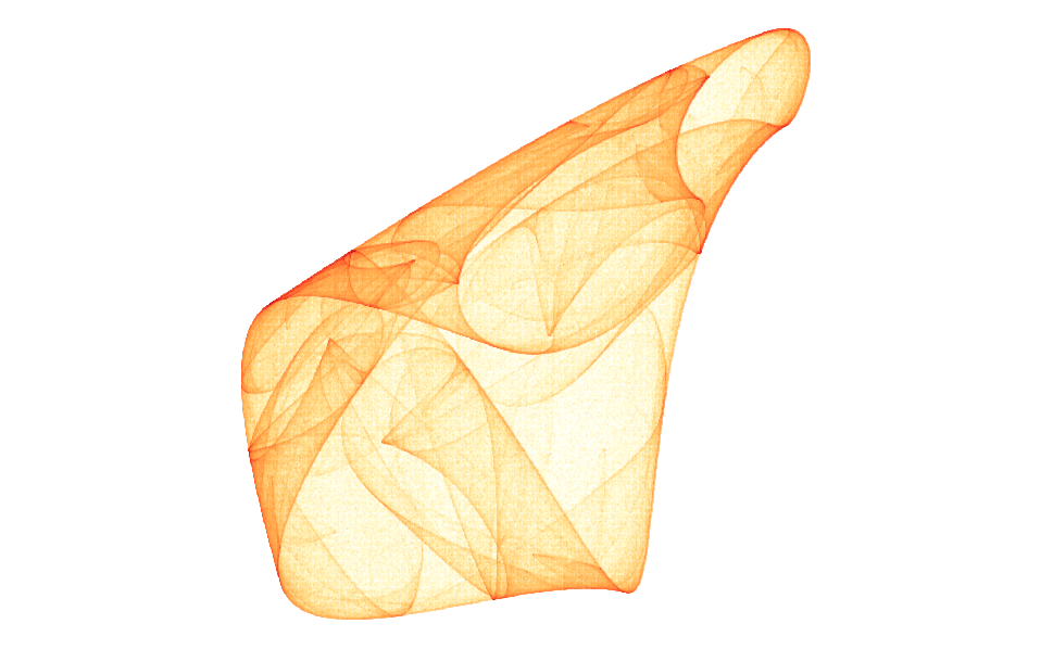
This code utilizes the ggplot2 package to generate a scatter plot of the data stored in the dataframe d. Each point in the plot is represented by its coordinates on the x and y axes. Additionally, the points are styled based on two additional variables:
The alpha aesthetic is mapped to the square root of the variable n, controlling the transparency of the points. This transformation is commonly used to improve the visual perception of density in the plot.
The color aesthetic is mapped to the logarithm of the variable n, determining the color of the points on a continuous scale. This transformation is often used to emphasize differences in magnitude while compressing the color scale.
Furthermore, the code applies additional formatting to the plot:
The scale_alpha_continuous function specifies the range of transparency values to be between 0 and 1, with no upper limit.
The scale_color_distiller function adjusts the color palette to a sequential palette named ‘YlOrRd’, which ranges from yellow to orange to red.
Finally, the coord_equal function ensures that the x and y axes are scaled equally, preserving the aspect ratio of the plot.
In our pursuit to understand the complex dynamics of 2D quadratic maps, we embarked on a systematic journey akin to navigating a maze of possibilities. Beginning with the generation of a vast array of trajectories, we identified promising patterns hinting at chaotic behavior. By delving deeper into selected trajectories through extensive iterations, we uncovered hidden complexities and nuances. Refining our focus on the most captivating trajectories, we meticulously styled and refined them into visual representations that captured the essence of chaos and beauty. In the end, our expedition yielded a collection of trajectories that serve as testaments to our journey—a journey characterized by curiosity, exploration, and an unwavering commitment to understanding.
Strange Attractors: Creating Patterns in Chaos by Julien C. Sprott
Automatic Generaton of Strange Attractors by Julien C. Sprott
A. A. Chernikov R. Z. Sagdeev and G. M. Zaslavsky: “Chaos: How Regular Can it Be?” (Physics Today 27 November 1988).
J. P. Crutchfield J. D. Farmer N. H. Packard and R. S. Shaw: “Chaos” (Scientific American 255 46 December 1986)

---
title: "Exploring Strange Attractors"
subtitle: "A Computational Journey through Parameter Spaces"
date: 2024-02-10
author: "Abhirup Moitra"
format:
html:
code-fold: true
code-tools: true
editor: visual
categories: [Mathematics, Physics]
image: m-sc.jpg
---
{fig-align="center" width="344"}
::: {style="color: navy; font-size: 18px; font-family: Garamond; text-align: center; border-radius: 3px; background-image: linear-gradient(#C3E5E5, #F6F7FC);"}
**"The grand aim of all science is to cover the greatest number of empirical facts by logical deduction from the smallest number of hypotheses or axioms." - Albert Einstein**
:::
# **Exploring the Unpredictable**
This research article delves into the fascinating realm of strange attractors, as elucidated in Julien C. Sprott's seminal work. The availability of Sprott's book as a free downloadable resource has facilitated widespread exploration of these complex phenomena. Noteworthy features include a profusion of captivating imagery and accompanying source code, rendering the subject accessible to enthusiasts adept in basic programming. A key focus of this research lies in the exploration of strategies to navigate the vast parameter spaces inherent to strange attractors. Drawing insights from the techniques expounded in Sprott's text, the paper sheds light on methodologies to discern aesthetically pleasing patterns within these intricate systems. Central to our investigation is the implementation of a two-dimensional quadratic map, governed by a set of twelve parameters.
$$
\begin{align*}x_{n+1} &= a_1 + a_2 x_n + a_3 x_n^2 + a_4 x_n y_n + a_5 y_n + a_6 y_n^2 \\y_{n+1} &= a_7 + a_8 x_n + a_9 x_n^2 + a_{10} x_n y_n + a_{11} y_n + a_{12} y_n^2\end{align*}
$$
Through judicious selection and manipulation of these parameters, we embark upon a visual journey, culminating in the generation of captivating images. The paper offers insights into the nuances of parameter selection and its profound impact on the resultant visualizations. By leveraging Sprott's foundational work and building upon it with novel implementations in the *R programming language*, this paper contributes to the ongoing discourse surrounding strange attractors. It underscores the symbiotic relationship between mathematical theory and computational implementation in unraveling the mysteries of chaotic dynamical systems. In conclusion, this research serves as a testament to the enduring relevance and beauty of strange attractors, offering both theoretical insights and practical methodologies for enthusiasts and researchers alike.
## **Computational Methods**
In order to generate an initial illustrative depiction, a deliberate selection of parameter values for the twelve variables was undertaken. The determination of 'suitable' values, a concept meriting further elucidation, was pivotal in this process. Subsequently, a series of computational steps were executed, culminating in the generation of visual representations elucidating the emergent patterns. These results were then meticulously plotted for comprehensive analysis and interpretation.
**1.1 Code**
```{r,message=FALSE,warning=FALSE}
library(tidyverse)
theme_set(theme_void() + theme(legend.position = 'none'))
# I will go parallel a little later; set up my computer for this
library(future)
library(furrr)
```
This code segment is written in R and serves to set up the environment for subsequent data visualization and parallel processing tasks.
1. **`library(tidyverse)`**: This line loads the tidyverse package, which is a collection of R packages designed for data manipulation and visualization. It includes popular packages such as ggplot2, dplyr, and tidyr.
2. **`theme_set(theme_void() + theme(legend.position = 'none'))`**: This line sets the default theme for plots using ggplot2 to a blank theme (**`theme_void()`**) with no axes or background, and also removes the legend from plots. This ensures that plots generated later will have a clean appearance without unnecessary clutter.
3. **`library(future)`**: This line loads the future package, which provides tools for parallel computing in R.
4. **`library(furrr)`**: This line loads the furrr package, which builds on top of future and provides a user-friendly interface for parallel programming in R.
The primary function, denoted as `quadratic_2d()`, is designed to accept a vector denoted as 'a', encapsulating the twelve parameters pertinent to the two-dimensional quadratic map. Additionally, this function requires an input pair comprising the coordinates along the x and y axes, designated as an $(x,y)$ pair, to compute and generate the subsequent step forward within the dynamical system.
**1.2 Code**
```{r}
quadratic_2d <- function(a, xn, yn) {
  xn1 <- a[1] + a[2]*xn + a[3]*xn*xn + a[ 4]*xn*yn + a[ 5]*yn + a[ 6]*yn*yn
  yn1 <- a[7] + a[8]*xn + a[9]*xn*xn + a[10]*xn*yn + a[11]*yn + a[12]*yn*yn

  c(xn1, yn1)
}
```
This code defines a function named **`quadratic_2d`**. This function takes three arguments: **`a`**, **`xn`**, and **`yn`**.
- **`a`** is expected to be a vector containing twelve parameters.
- **`xn`** represents the current value along the x-axis.
- **`yn`** represents the current value along the y-axis.
Within the function, two new variables **`xn1`** and **`yn1`** are computed using the supplied parameters **`a`** and the current coordinates **`xn`** and **`yn`** according to the formulas provided. These formulas represent the calculation of the next step forward in a two-dimensional quadratic map. Finally, the function returns a vector containing the newly computed values **`xn1`** and **`yn1`**.
We have further implemented a function, termed `iterate()`, to systematically traverse through iterations within the defined dynamical system. The `iterate()` function facilitates the accumulation of outcomes, yielding a comprehensive list of points visited throughout the execution of the map over a specified number of iterations. Utilizing a set of parameters, designated as 'a', this function orchestrates the generation of what is commonly referred to as the **Hénon map**, as delineated below.
**1.3 Code**
```{r,message=FALSE,warning=FALSE}
iterate <- function(step_fn, a, x0, y0, iterations) {
  x <- rep(x0, iterations)
  y <- rep(y0, iterations)

  for(n in 1:(iterations - 1)) {
    xy <- step_fn(a, x[n], y[n])
    x[n+1] <- xy[1]
    y[n+1] <- xy[2]
  }

  tibble(x = x, y = y) %>%
    mutate(n = row_number())
}

henon_a <- c(1, 0, -1.4, 0, 0.3, 0, 0, 1, 0, 0, 0, 0)
iterate(step_fn = quadratic_2d, a = henon_a,
        x0 = 0, y0 = 0, iterations = 5000) %>%
  ggplot(aes(x, y)) +
    geom_point(size = 0, shape = 20, alpha = 0.2) + # Plot a pixel for each point
    coord_equal()
```
This code defines a function named **`iterate`** and subsequently utilizes it to generate and visualize a trajectory within the Hénon map using the specified parameters.
The **`iterate`** function takes five arguments: **`step_fn`**, **`a`**, **`x0`**, **`y0`**, and **`iterations`**.
- **`step_fn`** represents the function responsible for computing the next step in the iteration process.
- **`a`** denotes the parameters governing the dynamical system.
- **`x0`** and **`y0`** signify the initial coordinates from which the iteration begins.
- **`iterations`** indicates the total number of iterations to perform.
Within the **`iterate`** function, two vectors **`x`** and **`y`** are initialized with repeated values of **`x0`** and **`y0`**, respectively. Subsequently, a loop iterates through each step, invoking the **`step_fn`** function to compute the next coordinates based on the parameters **`a`** and the current **`x`** and **`y`** values. These computed coordinates are stored in the **`x`** and **`y`** vectors for subsequent iterations.
Upon completion of the iteration process, a tibble (data frame) is constructed with columns **`x`** and **`y`**, representing the trajectory, and an additional column **`n`** denoting the iteration number.
The subsequent code snippet utilizes the **`iterate`** function to generate a trajectory within the Hénon map, specifically employing the parameters defined in the **`henon_a`** vector. The trajectory is initialized from the origin (0, 0) and spans 5000 iterations.
The resulting trajectory is then visualized using ggplot2, with each point represented as a pixel on the plot. The **`geom_point`** function is employed to plot the points, while **`coord_equal()`** ensures that the aspect ratio of the plot remains consistent. Additionally, the points are rendered with minimal size (**`size = 0`**) and transparency (**`alpha = 0.2`**), facilitating the visualization of the entire trajectory.
# **Algorithmic Analysis and Computational Insights**
In the context of a 2D quadratic map, it is imperative to acknowledge the intricate nature of parameter selection, wherein a staggering twelve parameters necessitate discerning choices. However, not all parameter configurations yield meaningful or visually captivating outcomes.
Distinct categories of plots emerge contingent upon the specific parameter combinations:
1. **Converging**: These plots depict trajectories culminating in fixed points, offering little in terms of visual intrigue or dynamical complexity.
2. **Run-away**: Characterized by trajectories spiraling towards infinity, these plots similarly lack substantive interpretive value.
3. **Chaotic**: Representing the focal point of interest, chaotic plots exhibit intricate, non-linear behavior, embodying the essence of dynamical complexity.
In pursuit of chaotic behavior, parameter values within a bounded range typically exhibit the greatest propensity for generating visually compelling results. Empirical observations suggest that parameter values ranging between -1.5 and 1.5, incremented by steps of 0.01, offer a favorable likelihood of inducing chaotic behavior. Nonetheless, even within this bounded domain, the sheer combinatorial magnitude remains daunting, with an estimated 10\^70 distinct parameter configurations.
To mitigate the arduous task of manually sifting through this vast parameter space, computational techniques can be harnessed. A fundamental understanding of chaotic systems reveals two salient characteristics:
1. **Divergence**: Nearby points within the system tend to diverge from each other over successive iterations, precluding convergence towards a fixed point.
2. **Finite Bounds**: Despite the tendency to diverge, trajectories within chaotic systems remain bounded, exhibiting periodic oscillations rather than unbounded divergence towards infinity.
Guided by these insights, an algorithmic approach emerges: iteratively track the trajectories of two adjacent points within the parameter space. At each iteration, evaluate the change in distance between these points and ascertain whether it increases or decreases. Subsequently, aggregate these observations over multiple iterations, discerning whether the average ratio of post-iteration to pre-iteration distances exceeds unity, indicative of divergent behavior. This algorithmic framework enables automated identification and characterization of chaotic parameter configurations, alleviating the burden of manual exploration within the parameter space.
In mathematical terms, let us define the parameter $L$ as follows:
$$
L = \sum_{l} \frac{\log_2 (d_n + 1)}{d_n / N}
$$
Here, $d$ represents the distance between two successive points, and $N$ denotes the total number of points evaluated. Notably, given the utilization of logarithmic transformations, our criterion for chaotic behavior hinges upon the condition $L>0$ (owing to the property that $2^0=1$).
Subsequently, upon satisfying the condition $L>0$ and observing that the $xy-$ coordinates do not exhibit unbounded growth (remaining within a finite range, for instance, within the interval $±$ one million), we identify a set of parameters exhibiting chaotic behavior. Let’s implement a function to calculate $L$.
**1.4 Code**
```{r}
L <- function(step_fn, a, x0, y0, iterations = 1000) {
  # Really, put the point nearby and see what happens
  nearby_distance <- 0.000001

  xy <- c(x0, y0)
  xy_near <- xy + c(nearby_distance, 0)

  # Collect the log distance ratios as we iterate
  sum_log_distance_ratios <- 0

  for (n in 1:iterations) {
    xy <- step_fn(a, xy[1], xy[2])
    xy_near <- step_fn(a, xy_near[1], xy_near[2])

    new_distance = sqrt((xy[1] - xy_near[1])^2 + (xy[2] - xy_near[2])^2)

    if (new_distance == 0) {
      # The points have converged
      return (-Inf)
    }

    if (abs(new_distance) == Inf) {
      # The points have run away
      return (Inf)
    }

    # Move near point after xy
    # We put the near point just behind in the direction that they differ
    angle = atan2(xy_near[2] - xy[2], xy_near[1] - xy[1])
    xy_near <- c(xy[1] + nearby_distance * cos(angle),
                 xy[2] + nearby_distance * sin(angle))


    sum_log_distance_ratios = sum_log_distance_ratios + log2(new_distance / nearby_distance)

  }

  sum_log_distance_ratios / iterations
}
```
1. This code defines a function named **`L`** that computes the value of the parameter $L$, as described earlier. The function takes five arguments: **`step_fn`**, **`a`**, **`x0`**, **`y0`**, and **`iterations`**, with **`iterations`** defaulting to $1000$. Within the function, a nearby distance variable is initialized to a very small value, allowing for the creation of a nearby point during the iteration process.
2. Subsequently, the function iterates through a loop for the specified number of iterations. At each iteration, it computes the distance between the current point and the nearby point, updates the nearby point using the **`step_fn`** function, and calculates the new distance between the updated points. If the distance between the points becomes zero, indicating convergence, the function returns negative infinity. Conversely, if the distance becomes infinite, indicating divergence, the function returns positive infinity.
3. Finally, the function computes the sum of the logarithmic distance ratios over all iterations and divides it by the total number of iterations to obtain the average value of $L$, which is then returned. Overall, this function encapsulates the algorithmic approach outlined earlier for assessing chaotic behavior within the dynamical system.
## **Screening and Iterative Analysis of Parameter Sets**
Applying this computational methodology to a selection of parameter sets, we aim to assess the chaotic behavior inherent within the Hénon map, as established in prior literature.
```{r}
L(quadratic_2d, henon_a, 0.01, 0.01)
```
When all parameters are set to zero, the iterative process converges to the fixed point located at the origin, denoted as $(0, 0).$
```{r}
L(quadratic_2d, rep(0, 12), 0.01, 0.01)
```
With the requisite components integrated into the computational framework, a comprehensive exploration ensues wherein a sizable array of parameter sets is randomly generated. From this pool, only those exhibiting characteristics indicative of chaotic behavior are selectively retained for further analysis.
**1.5 Code**
```{r,eval=FALSE}
set.seed(1)

df <- tibble(pattern = 1:1000) %>%
  mutate(a = map(pattern, ~ round(runif(12, -1.5, 1.5), 2))) %>%
  mutate(L_val = map_dbl(a, ~ L(quadratic_2d, ., 0, 0))) %>%
  filter(L_val > 0)

print(df)
```
This code segment initiates a computational procedure aimed at identifying parameter sets conducive to chaotic behavior within the context of a 2D quadratic map. The **`set.seed(1)`** function ensures reproducibility by fixing the random number generator seed.
Subsequently, a tibble named **`df`** is generated, containing a sequence of integers labeled as **`pattern`** ranging from 1 to 1000. Each integer is associated with a corresponding set of twelve parameters denoted as **`a`**, generated using the **`runif()`** function to randomly sample values within the interval \[-1.5, 1.5\], rounded to two decimal places.
The **`map()`** function from the **`purrr`** package is then employed to apply the **`quadratic_2d`** function iteratively to each parameter set **`a`**, alongside initial coordinates $(0, 0)$, to compute the value of the parameter $L$. This results in the creation of a new column **`L_val`** within the dataframe **`df`**, containing the calculated values of $L$.
Subsequently, the dataset is filtered to retain only those parameter sets for which the computed $L$ value exceeds zero, indicative of chaotic behavior.
Finally, the resulting dataframe **`df`** is printed to the console, providing a tabular representation of the parameter sets that exhibit chaotic dynamics within the 2D quadratic map.
## **Iterative Examination of Parameter Sets in 2D Quadratic Maps**
In this analysis, we identify a subset of 17 candidate parameter sets characterized by an $L$ value exceeding zero, indicative of potential chaotic behavior within the dynamical system. While it remains plausible that some of these sets may exhibit unbounded divergence with further iterations, our initial screening process effectively reduces the pool of parameter sets necessitating computation and inspection.
To harness the potential of these promising parameter configurations, a subsequent iteration is conducted with an increased number of iterations. Additionally, to facilitate comparative analysis and visualization, the $xy-$ coordinates are normalized to a range from $0$ to $1$, ensuring uniform scaling across all plotted trajectories
**1.6 Code**
```{r,eval=FALSE,warning=FALSE,message=FALSE}
normalize_xy <- function(df) {
  range <- with(df, max(max(x) - min(x), max(y) - min(y)))

  df %>%
    mutate(x = (x - min(x)) / range,
           y = (y - min(y)) / range)

}

render_grid <- function(df, iterations) {
  df %>%
    mutate(xy = map(a, ~ iterate(quadratic_2d, ., 0, 0, iterations))) %>%

    # Remove those who have grown very large / might run away
    filter(map_lgl(xy, function(d) with(d, all(abs(x) + abs(y) < 1e7)))) %>%

    mutate(xy = map(xy, normalize_xy)) %>%

    unnest(xy) %>%
    ggplot(aes(x, y)) +
      geom_point(size = 0, shape = 20, alpha = 0.1) +
      coord_equal() +
      facet_wrap(~ pattern)
}

df %>%
  render_grid(5000)
```
{fig-align="center"}
This code performs two main tasks: normalizing $xy-$ coordinates and rendering a grid of plots representing trajectories of parameter sets in a 2D quadratic map.
1. **`normalize_xy` function**: This function takes a dataframe **`df`** containing $xy-$ coordinates and normalizes these coordinates to a range from 0 to 1. It first calculates the range of values in both $x$ and $y$ dimensions. Then, it updates the dataframe by transforming each $x$ and $y$ coordinate using the formula $\frac{x- \text{min}(x)}{\text{range}}$ and $\frac{y-\text{min(y)}}{\text{range}}$, respectively.
2. **`render_grid` function**: This function renders a grid of plots representing trajectories of parameter sets in a 2D quadratic map. It takes two arguments: **`df`**, a dataframe containing parameter sets, and **`iterations`**, the number of iterations to compute the trajectories.
- It first computes the trajectories for each parameter set using the **`iterate`** function.
- Next, it filters out trajectories that have grown very large or might run away, ensuring that only stable trajectories are plotted.
- Then, it normalizes the $xy-$ coordinates of each trajectory using the **`normalize_xy`** function.
- Finally, it creates a grid of plots using ggplot2, with each plot representing the trajectory of a parameter set. The plots are arranged in a grid format, with each row corresponding to a different parameter set (**`pattern`**).
3. The last part of the code applies the **`render_grid`** function to the dataframe **`df`** with a specified number of iterations (5000), generating and displaying the grid of plots representing the trajectories of parameter sets in the 2D quadratic map.
Despite the presence of some trajectories exhibiting periodic behavior deemed less visually appealing, we proceed to render one trajectory with enhanced quality for thorough analysis:
**1.7 Code**
```{r,eval=FALSE}
#pattern 423
df %>%
  filter(pattern == 423) %>%
  render_grid(100000)

#pattern 683
df %>%
  filter(pattern == 683) %>%
  render_grid(100000)

#Pattern 694
df %>%
  filter(pattern == 694) %>%
  render_grid(100000)

#Pattern 75
df %>%
  filter(pattern == 75) %>%
  render_grid(100000)
```
1. **Pattern 423:** This code filters the dataframe **`df`** to retain only the observations corresponding to **`pattern`** number 423. It then calls the **`render_grid`** function with this filtered subset of data and a specified number of iterations (100,000). The **`render_grid`** function generates and renders a plot representing the trajectory of parameter sets associated with pattern 423 in the 2D quadratic map, using a larger number of iterations to capture finer details of the trajectory.
2. **Pattern 683:** This code selects a subset of data from the dataframe **`df`** where the **`pattern`** variable is equal to 683. It then proceeds to render a grid of plots representing trajectories associated with this specific pattern, using a large number of iterations (100,000) to capture intricate details of the trajectory behavior.
3. **Pattern 694:** This code filters the dataframe **`df`** to extract observations corresponding specifically to **`pattern`** number 694. Subsequently, it generates a grid of plots representing trajectories associated with this pattern. The function utilizes a significant number of iterations (100,000) to ensure thorough examination and capture intricate details of the trajectory dynamics.
4. **Pattern 75:** This code filters the dataframe **`df`** to extract observations corresponding exclusively to **`pattern`** number 75. Subsequently, it generates a grid of plots representing trajectories associated with this specific pattern. Utilizing a substantial number of iterations (100,000), the function aims to comprehensively analyze and depict the intricate details of the trajectory dynamics for this particular pattern
::: {layout-nrow="2"}


:::
# **Enhancing Visualization and Accelerating Computation through Parallelization Techniques**
We employ a flexible approach to adjust the rendering of identified patterns, aiming to enhance visualization effectiveness. A notable technique involves aggregating individual points into grid-based 'bins,' facilitating efficient visualization by quantifying the density of points within each cell. This method allows us to map the count of points to color and transparency values, offering insights into the spatial distribution of trajectories.
To expedite computational processing, we implement parallelization techniques for data generation. By distributing the iterations evenly across the cores of the CPU, computational workload is efficiently managed. Additionally, we introduce slight variations in starting points for each thread, resulting in parallel execution of iterations across multiple cores. Given the nature of attractors to converge trajectories towards more frequently visited regions regardless of initial starting points, the concurrent execution of multiple paths remains imperceptible.
**1.8 Code**
```{r,eval=FALSE,message=FALSE,warning=FALSE}
render_print_data <- function(a, iterations, gridsize) {
  CPU_cores <- parallel::detectCores()

  tibble(thread = 1:CPU_cores) %>%
    mutate(x0 = runif(length(thread), -0.1, 0.1),
           y0 = runif(length(thread), -0.1, 0.1)) %>%
    mutate(xy = future_pmap(., function(x0, y0, ...) iterate(quadratic_2d, a, x0, y0, iterations / CPU_cores))) %>%
    unnest(xy) %>%

    # Normalize
    mutate(range = max(max(x) - min(x), max(y) - min(y))) %>%
    mutate(x = (x - min(x)) / range,
           y = (y - min(y)) / range) %>%

    group_by(x = round(x * gridsize) / gridsize,
             y = round(y * gridsize) / gridsize) %>%
    summarize(n = n())
}

df.chosen <- df %>%
  filter(pattern == 694)

d <- render_print_data(df.chosen$a[[1]], 2000000, 1000)

print(head(d))
```
Concluding this phase, meticulous attention is directed towards refining the visual representation of the data. The adjustment of image density is meticulously executed through the transformation of the 'alpha = n' variable, employing techniques such as logarithmic scaling, square root transformations, or cubic root adjustments. This endeavor necessitates a methodical trial-and-error approach to ascertain the optimal transformation method conducive to enhancing the clarity and interpretability of the visual output.
**1.9 Code**
```{r,eval=FALSE}
d %>%
  ggplot(aes(x, y)) +
    geom_point(aes(alpha = sqrt(n), color = log(n)), size = 0, shape = 20) +
    scale_alpha_continuous(range = c(0, 1), limits = c(0, NA)) +
    scale_color_distiller(palette = 'YlOrRd', direction = 1) +
    coord_equal()
```
{fig-align="center" width="484"}
This code utilizes the **`ggplot2`** package to generate a scatter plot of the data stored in the dataframe **`d`**. Each point in the plot is represented by its coordinates on the x and y axes. Additionally, the points are styled based on two additional variables:
1. The **`alpha`** aesthetic is mapped to the square root of the variable **`n`**, controlling the transparency of the points. This transformation is commonly used to improve the visual perception of density in the plot.
2. The **`color`** aesthetic is mapped to the logarithm of the variable **`n`**, determining the color of the points on a continuous scale. This transformation is often used to emphasize differences in magnitude while compressing the color scale.
Furthermore, the code applies additional formatting to the plot:
- The **`scale_alpha_continuous`** function specifies the range of transparency values to be between 0 and 1, with no upper limit.
- The **`scale_color_distiller`** function adjusts the color palette to a sequential palette named 'YlOrRd', which ranges from yellow to orange to red.
- Finally, the **`coord_equal`** function ensures that the x and y axes are scaled equally, preserving the aspect ratio of the plot.
# **Conclusion**
In our pursuit to understand the complex dynamics of 2D quadratic maps, we embarked on a systematic journey akin to navigating a maze of possibilities. Beginning with the generation of a vast array of trajectories, we identified promising patterns hinting at chaotic behavior. By delving deeper into selected trajectories through extensive iterations, we uncovered hidden complexities and nuances. Refining our focus on the most captivating trajectories, we meticulously styled and refined them into visual representations that captured the essence of chaos and beauty. In the end, our expedition yielded a collection of trajectories that serve as testaments to our journey—a journey characterized by curiosity, exploration, and an unwavering commitment to understanding.
# **See Also**
- [**Beauty in the Midst of Chaos**](https://abhirup-moitra-mathstat.netlify.app/chaosR/chaos-butterfly/)
- [**Bifurcation and Beginning of Chaos**](https://abhirup-moitra-mathstat.netlify.app/chaosR/bifurcation/)
# **References**
1. *Strange Attractors: Creating Patterns in Chaos* by [Julien C. Sprott](https://sprott.physics.wisc.edu/sprott.htm)
2. [Automatic Generaton of Strange Attractors by Julien C. Sprott](https://sprott.physics.wisc.edu/pubs/paper203.pdf)
3. A. A. Chernikov R. Z. Sagdeev and G. M. Zaslavsky: "Chaos: How Regular Can it Be?" (*Physics Today* 27 November 1988).
4. J. P. Crutchfield J. D. Farmer N. H. Packard and R. S. Shaw: "Chaos" (*Scientific American* **255** 46 December 1986)
{fig-align="center" width="363"}